GField Mapper User Manual

GField Mapper Pro User Manual

GField Mapper Pro

User Manual GField Mapper Pro application is an Android-based mobile module designed to do geological mapping significantly easy, saving time and efforts during post- processing. While primarily targeted at exploration and mapping geologists, it can also be effectively utilized by related professionals — such as geophysicists, engineering geologists, and environmental scientists — whose work relies on creating maps and documenting profiles. Additionally, the app enables high-quality, accurately georeferenced digitization of existing maps. For optimal results, we recommend using the app on tablets, though standard smartphones will also work; in both cases, we advise using at least a basic, budget-friendly stylus.

App Features Description:

The main toolbar (the vertical bar on the left side of the screen)

The buttons on this toolbar perform the following functions (from top to bottom):

"My Projects" allows you to create, import, and delete Projects, which are multi-layered maps with their own styling elements.

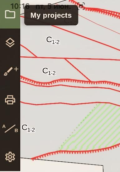
Opening the project list and drawing a boundary

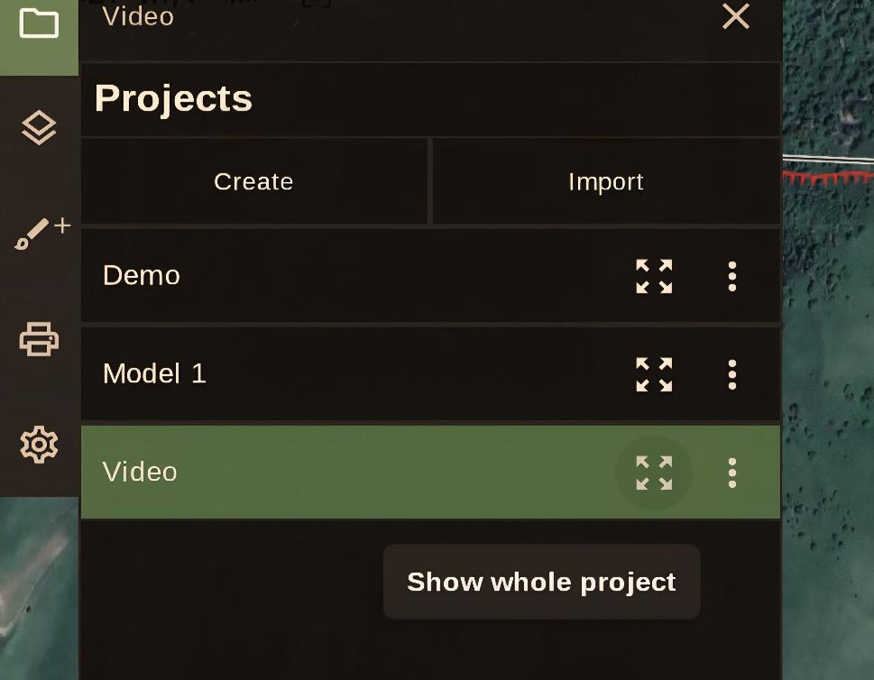
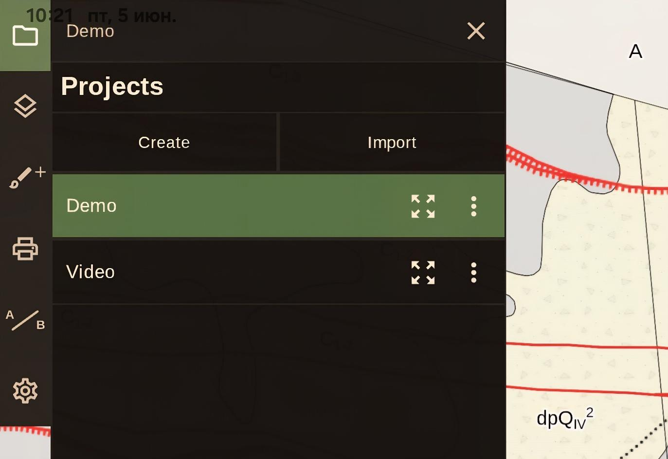
Clicking this button opens an additional window. If you have previously created or imported projects, they will be displayed here as a list. Clicking the name of any project in the list makes it the active project: its title turns green, and its multi-layered map is loaded and displayed in the main application window (while the previous project is unloaded).

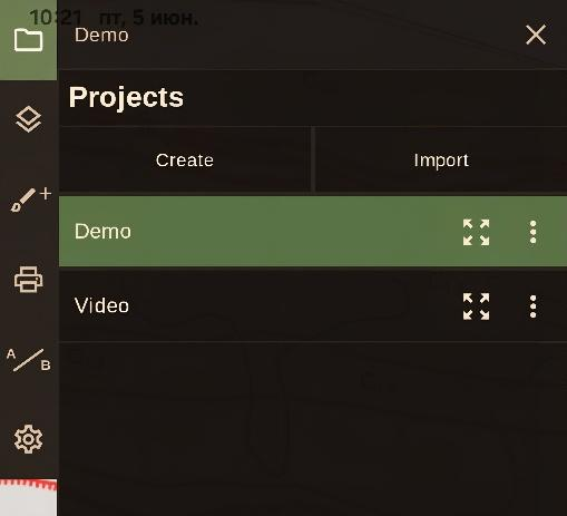
Clicking the "Create" button opens the "Add Project" window. Enter the name for your new project here:

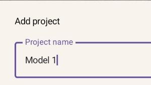
You can also set the boundaries of your new project in this window. Here are the available methods:

• 1. Click to "Tap Boundary" button and sequentially place clicks on the map to pin the corner points of the project boundary (work area or license area). Any of the created boundary nodes can be moved: simply select it (it should turn orange) and drag it to the desired location.

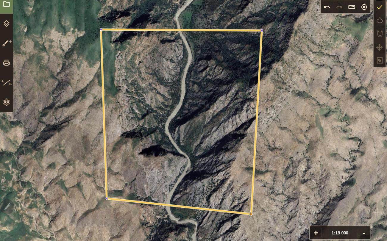
Confirming boundaries and importing project frames

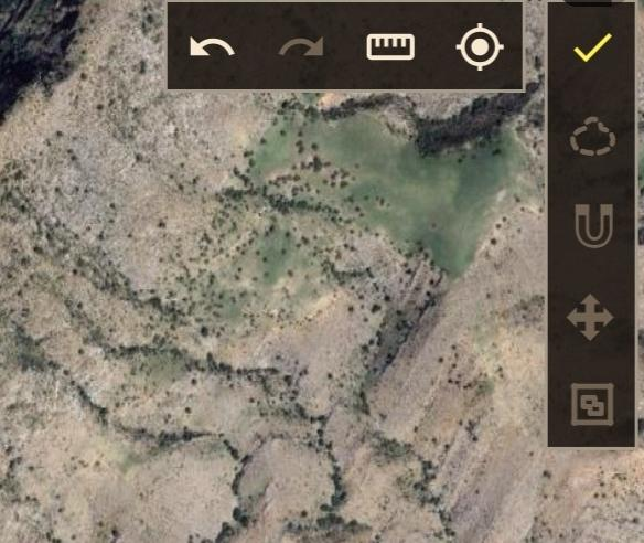
To confirm and finish the manual editing of the project boundary, click the yellow checkmark in the top-right corner of the screen...

after that, the settings window of new project reopens, where you can correct the frame node coordinates with actual (exact) numerical values, if known they.

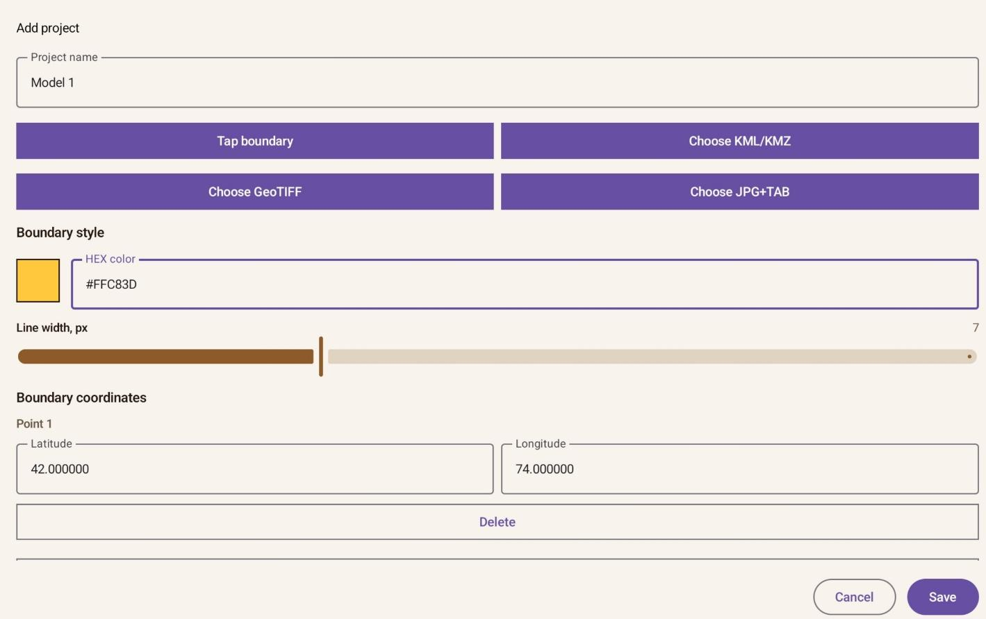
• 2. If you have a KML/KMZ file with a project boundary, you can use it. To do this, when creating a project in the “Edit Project” window, click the "Select KML/KMZ" button and choose the corresponding file on your device. It must be in your file directory, so we recommend creating a separate folder on your device in advance, named according to the project name.
• 3. Also, to set a boundary, you can select a georeferenced GeoTIFF raster, the borders of which will become the project frame. To do this, download the file to your device and, when creating a project, click on the “Select GeoTIFF” button.

Boundary sources, coordinates, and colors

• 4. In addition, you can define the project boundary by selecting a georeferenced JPG raster with an accompanying TAB file. The boundaries of the raster will be used as the project boundary. To do this, select the corresponding JPG and TAB files as a pair and upload them to your device by clicking the "Select JPG+TAB" button.
• 5. If you know the exact coordinates of all corners of the project frame, you can type them numerically, bypassing all the procedures described above. To do this, use the "Add coordinate point" button at the bottom of the “Create project” window and enter the coordinates of the corner points numerically, one by one.

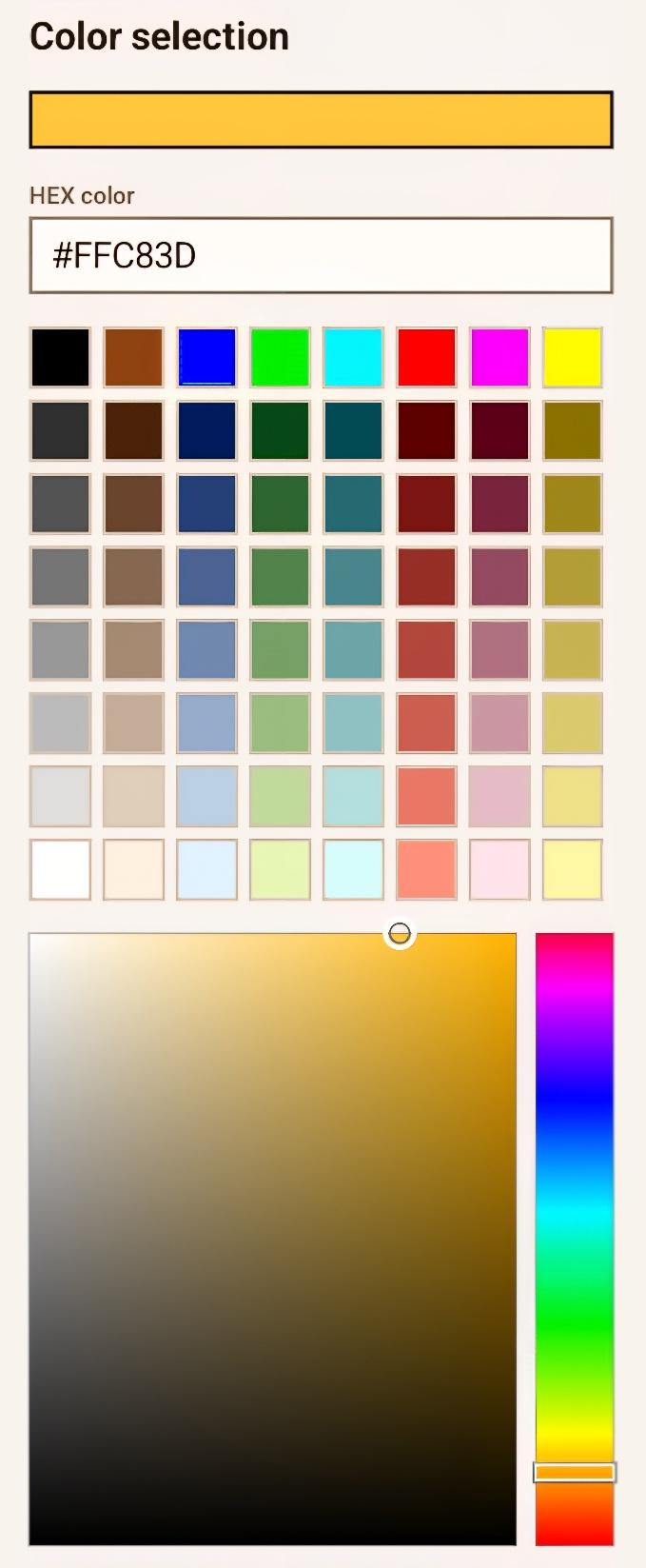
To change the color of the boundary line, click on the color square to choose one of 64 preset colors or choose a color from the full palette, or define an exact hue by typing its hex code.

Saving projects and project commands

Use the 'Line thickness, px' slider to set the boundary line thickness in pixels.

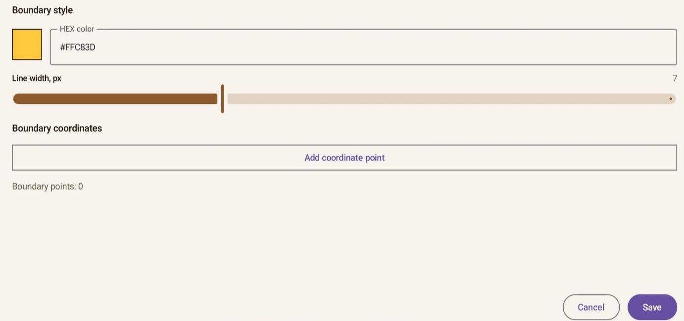
Next, click the "Save" button in the bottom right, and your new project is created and will appear in your project list.

To the right of the selected project name in the list, there is a "Show whole project" button. Clicking it fits the project frame to your device screen.

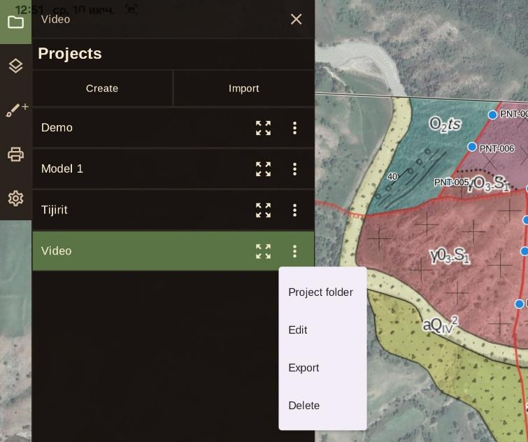
Clicking the button "⋮" on the right opens a command submenu:

Project folders, export, import, and deletion

• “Project Folder”: Tap this option to specify a location on your device or on an external memory card installed in the device that will be used as the “Project Folder”. If the folder does not already exist, it will be created automatically and assigned the project name. Exported project files, as well as point attachments, will be saved to this folder automatically as they are created or added. For attachments associated with a specific point, the application will automatically create a separate subfolder named after that point. • "Edit", clicking which takes you to the familiar Edit Project window, where you can modify the project settings; • "Export", clicking on it allows you to export the project to file named "project_name export_date export_time.gfield.zip". To save it, we recommend creating a separate folder on your device in advance, named according to the project; • “Delete" - on click, it permanently deletes the project.

If you need to add an existing project to the App, or if your device malfunctions and you have to reinstall the App (by the way, don't forget to export your project periodically as you fill it with data; this will be a lifesaver in the event of a total crash, which is highly unlikely but not impossible :-)), you can import a project saved on your device. To do this, use the "Import" button in the "Projects" window.

By clicking the Import button, the Select File to Import dialog opens. Click Select and specify the path to the project archive (.zip) file, which must already be stored on your device.

In the file selection window, simply tap the .zip archive with the stylus. This opens a dialog titled Select Folder for Project Storage, displaying the following message: the project folder will be created inside the folder you select. The original .zip archive, all future .zip archives you create, and the Attachments subfolders associated with points will be stored there.

A folder selection window then appears. Choose the directory in which the Project Folder should be created and click Use This Folder in the lower right corner. The application will automatically create a Project Folder named after the project, move the archive file into that folder, extract the point subfolders and their associated attachments from the archive, and then return to the main application window. The newly imported project will immediately appear in the project list.

Creating and working with layers

Lesson 2. Creating and working with layers

As with any GIS, the app is designed for creating objects in different layers. Layers higher in the list appear on top of those below them. Keep this in mind and set your layer order correctly.

The "Layers" button in the left vertical menu allows you to create, import, and delete layers for the active project's map, as well as change the order of layers and modify their properties. Clicking this button opens the "Layers" window, which displays the layers of your project. You can reorder layers in the list by simply dragging and dropping them. Clicking a layer's name activates it and highlights it in green. After creating a new project, the following layers are automatically created in it:

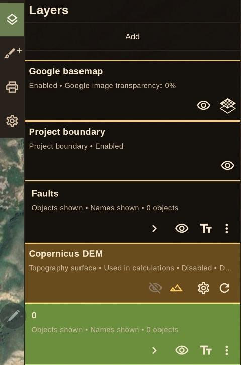
• “Google basemap” is an interactive layer of satellite imagery from the Google Earth web service. • “Project boundary” – the site limit or license area; • "Faults" layer is where your created or digitized faults will be stored, either as surface contours or direct projections of fault planes onto the surface; we will explain this in more detail later; • “Copernicus DEM” is an isoline layer for the basemap of the Copernicus web service. It is rather coarse and does not reflect the terrain perfectly. It is preferable to use your own, more accurate topographic basemap if you have one; we will cover this in more detail a bit later; • “0” – a fallback user layer where objects you create are placed if the target layer wasn't selected as active at the moment of creation (if you've lost something, look here).

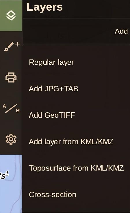
Clicking the "Add" button opens a list of available options for creating a new layer. All files to be uploaded must be stored on your device; please create a separate folder for your project for this purpose.

Layer types and layer control buttons

• "Regular layer" – create a new empty layer. Here, you only need to set its name; • «Add JPG+TAB» - import a georeferenced raster and create a separate layer for it. This opens your file tree: select a JPG file and its corresponding georeferenced TAB file from your project folder; • "Add GeoTIFF" – import a georeferenced raster and create a separate layer for it. Select it in the project folder along with its corresponding TAB georeference file; • "Add layer from KML/KMZ" - import a vector layer. Select the file in the project folder; • "Toposurface from KML/KMZ" — import a vector layer containing the site's toposurface contours. Select the file from your project folder. The layer created this way will later be used by the application to generate breaklines. If the user does not create their own base topography layer, the relatively coarse Copernicus DEM layer will be used instead; • "Cross-section" — to proceed with the construction of geological cross-sections; we will cover this topic later.

The layers are equipped with control buttons, which are located in the layer's rectangle below its name. Here are the functions of these buttons:

• open the list of features contained in this layer;
• show/hide layer;
• adjust raster layer visibility (available only for raster layers);
• show/hide layer feature labels;
• opens a list of two functions: "Edit" option allows you to rename the layer and toggle the visibility of the layer objects and their labels, while "Delete" allows you to delete the layer completely (the "Faults" and "Copernicus DEM" layers cannot be deleted);
• remove the imported layer from the project (for imported layers only).

For toposurfaces, a dedicated "Adjust basemap" button is available. A yellow glowing icon on the right indicates that this layer is selected as the elevation source for calculations. In the pop-up window, you can change the color and line thickness of the toposurface base.

"Refresh data" for updates the elevation data in the "Copernicus DEM" layer. This option is available if new data is accessible in this web service and there is an active Internet connection.

Lesson 3. Functions of the Utility Menus

Before moving on to creating objects and working with them, we recommend familiarizing yourself with the application's utility menus.

Horizontal toolbar and selected-object tools

The first one is the Horizontal Menu located in the upper right corner of the screen.

It contains four buttons that perform the following functions (from left to right):

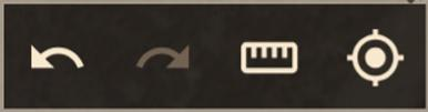
• Undo allows you to reverse (roll back) the last action. Multiple undo operations are supported. • Redo restores the previously undone action. Multiple redo operations are supported. • Ruler functions as a curvimeter. By clicking on the map, you can create a temporary path and measure its length. • My Location automatically centers the map on the user's current position. The current location is displayed as a blue circle with a white outline. Tapping this marker opens a small pop-up window showing the geographic coordinates of that point.

Spend a few minutes experimenting with these buttons to become familiar with their operation, as they can be very useful when working with the application.

The second utility menu is the Vertical Object Editing Menu, which appears in the upper right corner of the screen whenever an object is selected for editing. Below is a description of its buttons from top to bottom.

Clicking the Edit Properties button (gear icon) opens a dialog where the properties of the selected object can be modified. When a Contour is selected, either by clicking it on the map or choosing it from the layer object list, the Edit Contour dialog opens. It provides the following options:

• Enter or edit the contour name. Individual characters can be formatted using the B (Bold), I (Italic), x¹ (Superscript), and x₁ (Subscript) buttons. When these buttons are inactive, text is entered in the normal style. Special characters such as Є, š, č, as well as uppercase and lowercase Greek letters, can also be inserted using dedicated buttons. The contour name can optionally be displayed on the map, and its font size and color can be customized. • Configure the label size and color. The size is adjusted using a slider. To change the color, click the colored square on the left to open the Label Color dialog, where you can select one of the preset colors or fine-tune it using the color palette or the slider on the right. • Select the line geometry type: o Polyline: a line consisting of straight segments between nodes. o Spline: a smoothed curve connecting nodes with continuous curvature. • Select a line style from another project (Choose from project) or from Catalog, or create a custom style (Created by user), this will be discussed later in the lesson on creating Contours. You can also convert the contour into a polygon by enabling the Closed Contour option. • Adjust the contour line transparency using the Line Visibility slider. • Adjust the line thickness from 1 to 20 pixels using the Line Width slider. • Configure the Line Style Scale, which is important for displaying custom line styles correctly at the desired scale. • Configure the Fill and Hatch settings for closed contours (covered later). • Enable a black outline around the line by selecting Show Black Line Outline when Selected. • Discard changes using Cancel or save them using Save. • After saving, the application displays the notification "Contour saved locally."

The second button is Create Duplicate. It creates a copy of the selected contour and inserts it into the same layer with a slight offset from the original.

The third button, Copy to Clipboard, copies the selected object to the application's internal clipboard. When the clipboard contains an object, a fourth button becomes visible. Previously hidden, it allows you to Paste from Clipboard, inserting the copied object directly on top of the original without any offset. If two layers have been enabled for simultaneous editing (an optional feature available to the user), the copied object will be pasted into the second editable layer instead of the original one. In this

Contour editing and advanced commands

case, no duplicate is created in the first layer, and the application displays a notification indicating which layer received the pasted copy. The Selection Mode button (lasso icon) is available only when a contour is selected and you want to edit its nodes. It allows you to draw a lasso around multiple nodes of the contour so that they can be selected and deleted simultaneously The next button is Snap to Closest Vertex (magnet icon). This function is available while drawing a line. When enabled, each new node can automatically snap to a node belonging to another line or contour. The button is active only while the contour is still being drawn and has not yet been closed.

The Move Contour button allows the entire contour (line) to be repositioned. By default, moving a contour as a whole is disabled. However, all other editing operations, such as node editing, splitting, cutting, and similar actions, remain available without activating this function.

The Group Selection button allows multiple objects within the current editable layer to be selected at once. This is useful when you want to delete several objects simultaneously or move them to another layer. To activate this mode, click the button once. It will turn yellow and remain active until clicked again, at which point it returns to white. When Group Selection is enabled:

• selected contours display their nodes on the map; • selected objects in the layer object list are highlighted in bright green.

The three-dot button opens a list of additional commands. From top to bottom, these commands perform the following functions.

• The Continue Contour command allows you to resume drawing a line if it was interrupted accidentally. After selecting this command, drawing continues from the last existing node. Because the application continuously saves your work automatically, the most recent editing state can usually be recovered even after an unexpected program restart. • The Insert Vertex command adds a new node to an existing line in situations where inserting it directly by clicking on the map is difficult or impossible. • The Move Vertex command allows the selected node to be repositioned when direct manipulation on the map is not practical. • The Delete Vertex command removes the selected node when deletion by clicking directly on the map is not possible. • The Copy Properties command transfers the styling and display properties from one contour to another. To use it:
• 1. Select the destination contour. 2. Choose Copy Properties. 3. Click the contour whose properties should be copied.

The destination contour inherits the source contour's line style and all associated parameters, as well as its fill and hatch settings.

• The Join Segments command combines two separate lines into a single line. The lines do not have to share a common node. If necessary, the application automatically creates a connecting segment between them. The resulting merged line inherits the properties of the first selected contour. • The Union command combines two closed polygons into one continuous object. The common boundary between the polygons is removed, and the newer polygon inherits the properties of the older one. • The Subtract command subtracts one polygon from the currently edited polygon when the two overlap. The boundary of the subtracted polygon becomes part of the resulting shared boundary between the modified geometries. • The Split command splits a contour using either another closed polygon or an open line. As a result, the edited contour is divided into two or more separate parts. Unwanted fragments can

Editing points, structural elements, and faults

then be removed using the Delete command. Contours from different layers may participate in the operation, provided that the second layer has also been designated as editable. The application supports simultaneous editing of up to two layers. • The Move to Layer command transfers a contour from one layer to another. First select the contour, invoke the command, and then specify the destination layer.

The final button in the toolbar, Delete (trash bin icon), permanently removes the selected object.

Editing Other Object Types

The functionality described above applies primarily to Contours. However, the application supports three additional object types: Points, Strike and Dip Elements, and Faults, each of which has its own editing features.

Editing Points

When editing Points, the same editing menu used for Contours is displayed. However, some buttons are inactive because the corresponding operations are either unnecessary or not applicable to Point objects.

The following buttons remain available and perform the same functions as for Contours:

• Create Duplicate • Copy to Clipboard • Paste from Clipboard • Group Selection • Delete

Clicking Edit Properties (gear icon) opens a dialog where you can:

• view the point coordinates; • edit the point name; • adjust the label font size; • choose whether the point name should be displayed on the map by enabling the corresponding checkbox; • add or edit a comment; • select a point symbol from another project or from the Catalog, or create or edit symbol (this will be covered later in the lesson on creating Points); • specify the symbol color; • set the symbol size within a range of 1 to 128 pixels.

For Points, the three-dot menu contains only two additional commands:

• Copy Properties • Move to Layer

Points can also have attachments associated with them. This functionality will be described in a later lesson.

Editing Structural Elements

When editing Strike and Dip Elements, the same editing menu is displayed as for Contours, although several commands are inactive because they are not applicable to this object type.

Shared style synchronization and fault editing notes

The following commands remain available and function identically to their Contour counterparts:

• Create Duplicate • Copy to Clipboard • Paste from Clipboard • Group Selection • Delete

Selecting Edit Properties (gear icon) opens a dialog that allows you to:

• choose the required Strike and Dip Element type from the available list; • specify or modify its dip azimuth numerically; • specify or modify its dip angle numerically; • set its display color; • adjust its display scale as a percentage, which is important for correct visualization at the intended print scale; • enable or disable the display of the dip angle value on the map; • specify the font size of the displayed dip angle, from 0 to 128 pixels.

Important Note

Please note that the application automatically synchronizes the visual properties of all objects that share the same name.

If you modify the properties of one such object, including:

• label styles, • line thickness, • line color, • fills, • hatch patterns,

the same changes will be applied simultaneously to all other objects with the identical name.

This feature can be extremely useful for maintaining a consistent map style. However, it should be used thoughtfully, keeping its global effect in mind.

Editing Faults

When editing Faults, a similar editing menu is displayed, providing many of the same general functions available for other object types.

However, the Edit Properties (gear icon) dialog contains several features that are specific to Fault objects and differs significantly from the corresponding dialog used for Contours.

These specialized options will be discussed in detail later, when we cover Fault creation and editing. As you will see, this is an extensive and particularly interesting topic in its own right.

Creating points

Lesson 4. Adding objects to layers: Creating Points and Strike and Dip Elements Let's move on to the next button in the left vertical menu.

"Add object" button enables the creation of new features in the active map layer of the current project.

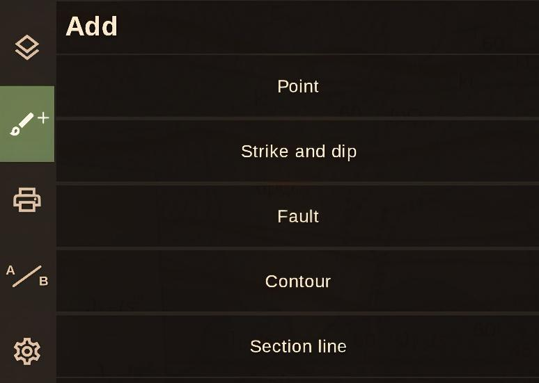
Creating Points

After selecting the "Point" object type, you need to click on the location on the map where you want to place the point. Next, the "Add Point" properties window of the newly created point opens. Here, you are prompted to set the point's properties sequentially:

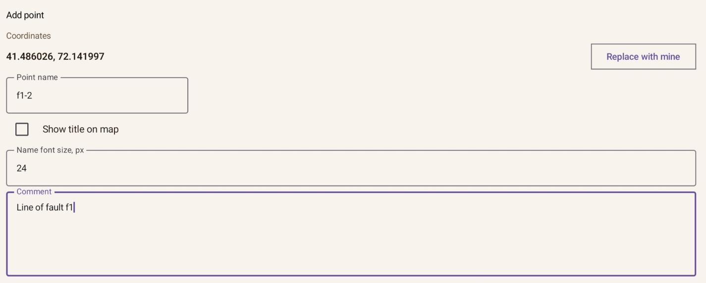
• "Replace with mine" - if you want to place a pin exactly at your current location, click this button and the coordinates of the pin will change;
• «Point name» – automatically generated by default with the prefix "PNT" and a number one higher than the previous point. The name can always be edited;
• «Show title on map» - enable/disable displaying the point's name on the map;
• «Name Font Size» — the font size used when displaying a point's name on the map;
• «Comment» - in this field, you can enter a brief text description of this point or its features;

Point symbols and the custom symbol constructor

• «Point symbol» - you can use the point symbol built into the Application; to do this, click the «No symbol» button, or select one from the built-in Application Catalog, the list of point types in which will gradually expand...

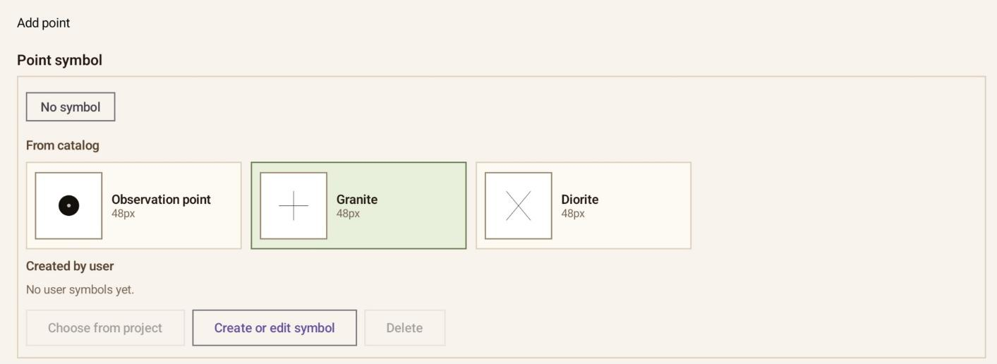
...or click the «Create or edit symbol» button, and in the opened window, specify the name and dimensions of the symbol...

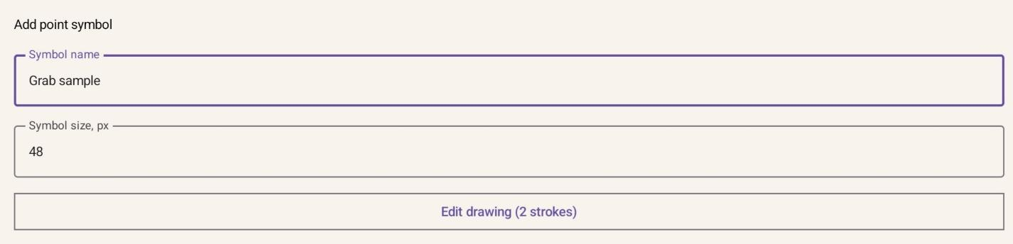
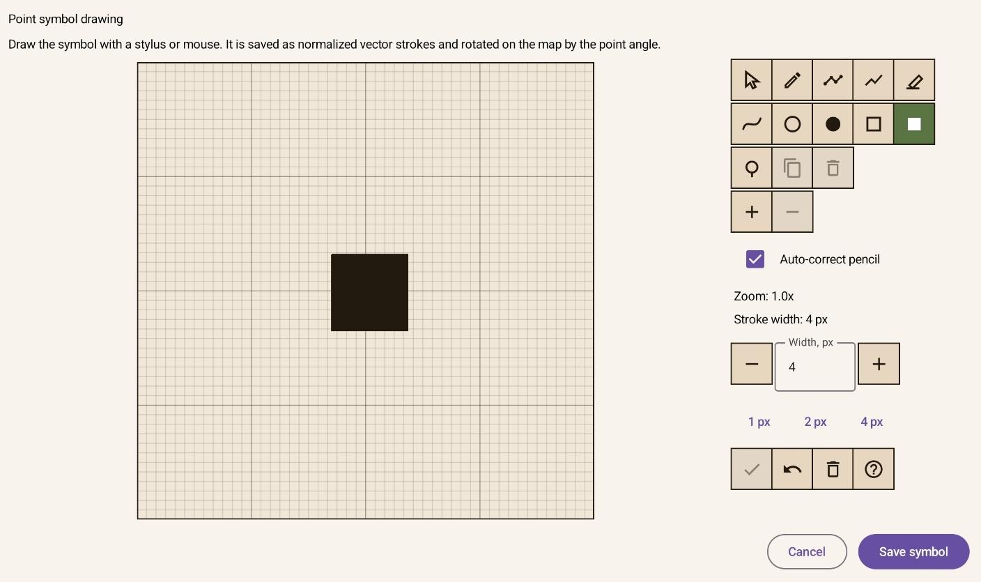
...and click the «Edit drawing» button to open the Constructor and create a new point symbol yourself.

Attachments and strike/dip elements

The Constructor is very user-friendly; if you have some experience with graphic editors, you can easily get the hang of it after trying it a few times.

Returning to the point properties we can assign. In addition to the above, at the bottom of the "Add Point" window, you can also configure:

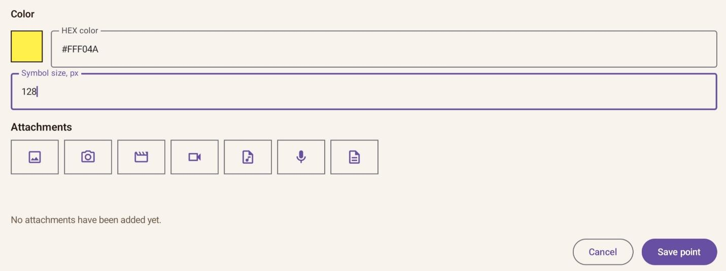
• «Color» - by clicking on the colored square, you can choose one of the 64 proposed colors or a color from the full palette. Here, you also have the option to set an exact color shade by entering its hexadecimal code; • «Symbol Size»: Defines the display size of the point symbol on the map. • «Attachments»: The buttons below allow you to attach existing files to the point or create and attach new ones. From left to right, the available attachment types are: image file, take photo, existing video file, record video, audio file, record audio, and document file. Once an attachment has been added, its name appears in the attachment list. Clicking the Open button allows you to view or play the selected attachment.

Creating Strike and Dip Elements

After selecting the object type «Strike and Dip Element» from the Add Object menu, click the location on the map where you want to place it. The Structural Element Properties dialog will then open. Here, you can review and, if necessary, modify the following properties:

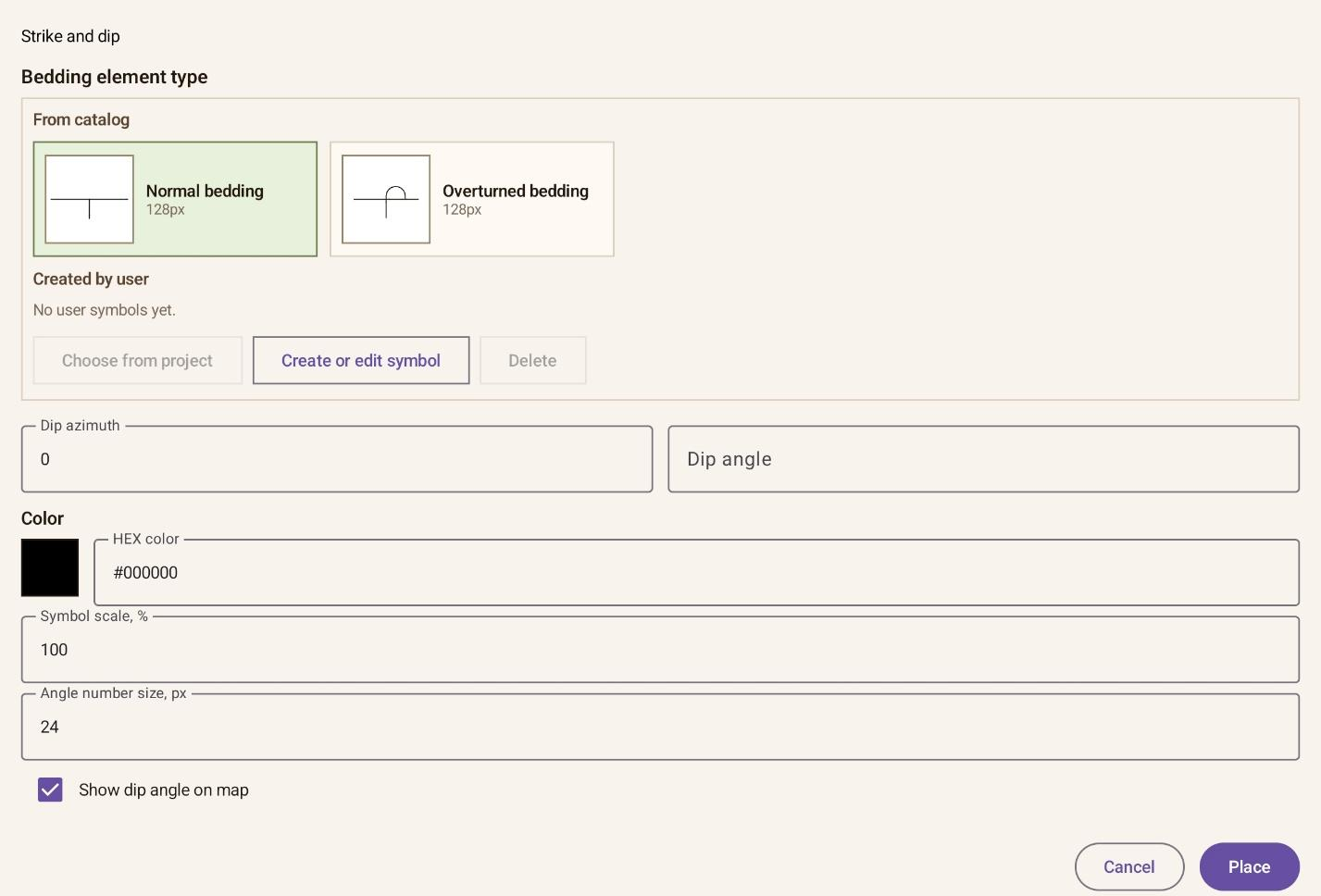
• «Bedding Element Type»: Select one of the structural element types available in the **Catalog**. If a suitable type is not available, you can create your own custom structural element. • Using «Choose from Project» button, you can import a custom strike and dip element created in another project (rather than one from the Catalog), provided that the other project is available in the application on your device. • «Delete» button serves as a utility function for removing a custom strike and dip element that you created or one imported from another project if it is no longer needed. Strike and dip elements provided by the Catalog cannot be deleted. • «Dip Azimuth»: Enter the dip azimuth manually. The strike and dip element will then be correctly oriented on the map. • «Dip Angle»: Enter the dip angle manually. The dip angle value will be displayed next to strike and dip element, and you can select and freely reposition this label on the map. • «Color»: Click the colored square to select one of the 64 preset colors or choose any color from the full palette. You can also specify an exact shade by entering its hexadecimal color code (see the color settings dialog described above). • «Symbol Scale, %»: Use this field to reduce the display size of the strike and dip element symbol. • «Dip Number Size»: Specifies the size of the dip angle numbers displayed on the map. • «Show Dip Angle on Map»: Enables or disables the display of the dip angle value on the map. • «Place»: Places the strike and dip element on the map.

Fault construction

Lesson 5. Adding Objects to Layers: Fault Construction

The fault construction functionality has been designed not only to enable users to draw the line representing the intersection of a fault plane with the ground surface in a two-dimensional map view, but also to preserve the fault plane itself in the application's memory as a three-dimensional object for subsequent use in 3D modelling. This represents an important step toward transforming the software into a fully featured Geographic Information System (GIS).

To create surface projections of faults, the application implements advanced methods for defining fault planes with their projections onto the terrain displayed instantly. Fault planes can be constructed from one, two, or three points, or directly from a line.

To create a fault, click the Add Object button (the brush icon with a + symbol) to open the Add menu, then select Fault. This will open the «Add Fault» dialog box, where you can sequentially specify the construction parameters and properties of the new fault.

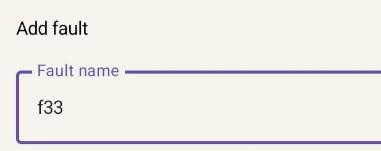
• 1) Fault Name is entered manually in the top field. We recommend assigning fault names with a distinctive prefix, such as “f” for fault, so that a typical name might be “f33”. The name can be edited at any time.

• 2. Definition Mode specifies how the fault will be constructed. A fault can be defined using one, two, or three points, or from a line. Each method has its own characteristics and use cases. To begin, create three collinear points on the map in any layer. If these are virtual reference points rather than actual field observation points, we recommend placing them in the auxiliary “0” layer.

Constructing a fault from points

We have now created three virtual points: PNT-031, PNT-032, and PNT-033. Next, we will construct a fault using these points.

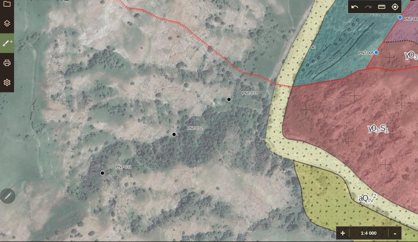
• Construction from a Single Point. Click the Show Points button to open a list of all points in your project. Select the desired point, for example PNT-033, then manually enter the required dip azimuth and dip angle in the corresponding fields. Next, scroll down the Add Fault dialog, choose the appropriate Geometry Type, Line Type, Color, Line Width, and Line Style Scale, and click Save Fault. The fault trace will then be displayed on the map.

The fault trace can be selected for editing, provided that the Faults layer is set as the active editable layer. Click Edit Properties to open the properties dialog, where you can modify the dip azimuth, dip angle, and other line attributes. After making the desired changes, click Save Fault to apply them and update the

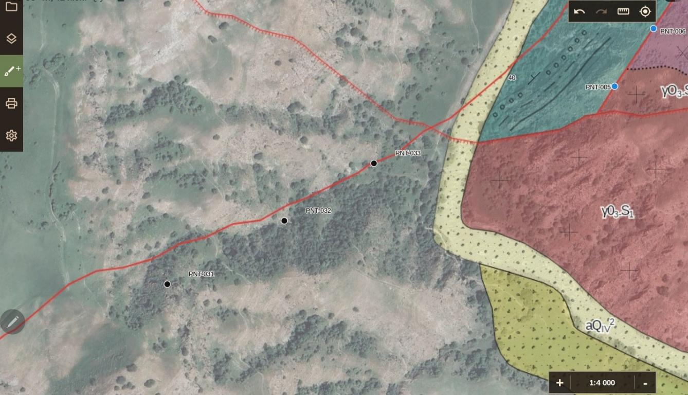
Two-point, three-point, and line-based faults

display on the map. This process can be repeated as many times as necessary until the required result is achieved.

• Construction from Two Points. In the Show Points list, select the two points you want to use. Then, in the Specified Dip Azimuth field, enter the approximate direction in which the fault plane dips. The exact dip azimuth will be calculated automatically based on the selected points. In the adjacent field, specify the Specified Dip Angle, which can later be adjusted to refine the fault trace. Click Save Fault to apply the settings and display the result on the map. You may modify the dip angle and save the fault repeatedly until the desired geometry is obtained. • Construction from Three Points. On the one hand, this is the simplest and most accurate method, because only one plane can be defined by three points in space, allowing the application to calculate the exact dip azimuth and dip angle automatically. On the other hand, if your topographic base is not sufficiently accurate, for example when using a Copernicus DEM, the resulting fault trace may not match reality as closely as desired. In such cases, the one-point or two-point methods may provide greater flexibility for adjusting the projected fault trace on the map. The procedure for construction from three points is the same as for the other methods, except that you select three points instead of one or two.

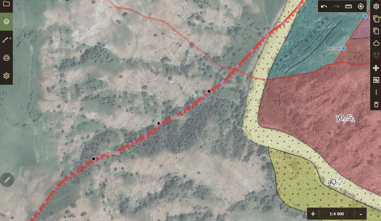
Projection lines of faults constructed from points on the map can be edited like regular contour lines, but corrections to the line are not reflected on the fault plane—keep this in mind when constructing cross-sections.

• The Line button allows you to construct a fault plane based on an arbitrary line drawn by the user on the map (we recommend using layer "0" for this). Clicking this button automatically creates a copy of the drawn line that has been snapped to the topography. The scale of this copy will be doubled or tripled to ensure it can be moved well beyond the boundaries of the project box, according to the dip azimuth and dip angle specified by the user. A plane is then constructed from the two resulting lines and subsequently trimmed by the project box. The resulting plane is unlikely to be perfectly smooth, but it will generally reflect the overall position of the fault in three-dimensional space and can be used for modeling. However, this method should be applied with caution and only in special cases, because if the original line is drawn incorrectly, the result can be highly unsatisfactory — something that will only become apparent later when constructing the 3D tectonic model.

Below, in the «Add Fault» window, the following functions are available:

• 3) Fault Projection. Geometry Type – selects how the fault projection is displayed on the surface of the area: Polyline – broken line, Spline – smooth curve.

Fault projection display properties

• 4) Line Type – depending on the type of fault and its reliability, select the appropriate line type from the catalog or from a set of user-defined types.
• 5) Create or Edit Line Type – opens a designer to create a custom line type for displaying such faults.
• 6) Color – clicking on the colored square allows you to choose one of the 64 suggested colors or a color from the full palette. You can also specify an exact color shade by entering its hexadecimal code.
• 7) Line Width – sets the thickness of the fault line.
• 8) Line Style Scale, % – this field allows you to reduce or enlarge the scale of the line type (this is important if, for example, you need to increase or decrease the size and number of tick marks or teeth on a thrust fault line so that they display correctly when printed at your desired scale).
• 9) Show Black Line Outline for Selected Line – toggles the display of a black outline along the fault line on the map.
• 10) Cancel – cancels fault creation without saving changes.
• 11) Save Fault – completes the fault creation process and opens the map with the new fault line displayed, which can then be edited using the "Edit Properties" button in the right vertical menu.

Creating contours

Lesson 6. Adding Objects to Layers: Creating Contours

The application allows you to draw object contours on the map using vector lines, preserving the 3D coordinates of each node, which enables their full use in 3D modeling later on. The operations that can be performed with contours are described in detail above in Lesson 3 "Utility Menu Functions".

To create a Contour, click the Add Object button (the brush icon with a + symbol) to open the Add menu, then click Contour. This will open the properties dialog for the new contour.

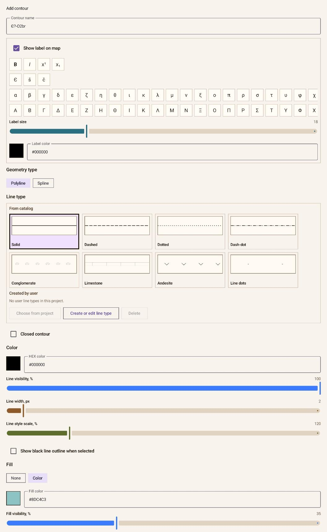
Here you need to set its properties sequentially:

Geological labels and contour styling

• 1) Contour Name is automatically assigned the same name as the previously created contour. The name can be edited at any time. 2) Show Label on Map enables or disables the display of the contour name on the map. 3) Below are four rows of buttons containing special symbols used to format geological formation indices in accordance with established standards and mapping conventions. These symbols can be inserted when entering the Contour Name in the field above. • First row: Text formatting buttons. Activate a button before typing the text to which the formatting should apply, then deactivate it to return to normal text entry. B (Bold) enables bold text, I (Italic) enables italic text, x¹ activates superscript mode, and x₁ activates subscript mode. • Second row: Special letter symbols (non-Latin) that are sometimes used in geological indices. • Third row: All lowercase letters of the Greek alphabet. • Fourth row: All uppercase letters of the Greek alphabet.

Text input is continuous; no intermediate saving is required. The result is immediately reflected in the label text input window. The final saving of the label occurs upon the general concluding command "Save Contour".

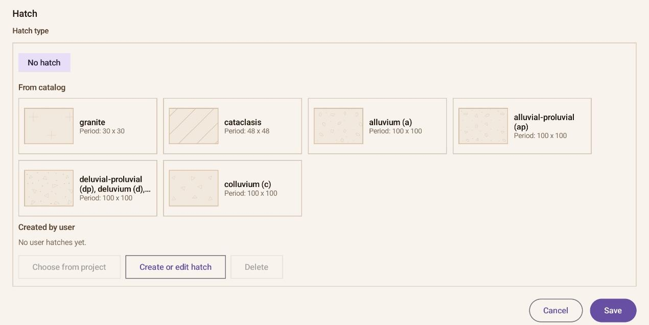
• 4. Label Size sets the font size used to display the contour name on the map. 5. Label Color allows you to select one of the 64 predefined colors or choose any color from the full palette by clicking the colored square. You can also specify an exact shade by entering its hexadecimal color code. 6. Geometry Type determines how the contour is displayed: Polyline (segmented line) or Spline (smooth curve). 7. Line Type can be selected either from the application's built in Catalog (whose collection of predefined line styles will be expanded over time and cannot be modified) or from a User-defined line type. A user- defined line type can be imported from another project stored on your device, provided that project is open. To do this, click Choose from Project, choose the desired project from the list of open projects, then select the required custom line types and click Done. The selected line types and their previews will appear on the left. 8. If you need a custom line style, click Create or Edit Line Type. In the dialog that opens, assign a Line Type Name, set the Pattern Scale in both the horizontal and vertical directions, then click Edit Repeated Line Fragment to open the editor and design the repeating pattern that will be drawn along the contour. You can cancel the operation with Cancel or save it with Save Pattern. 9. To modify an existing user-defined line type, select it by clicking its preview rectangle, then click Create or Edit Line Type and make the required changes. 10. To remove a user-defined line type from the project, select it by clicking its preview rectangle and then click Delete. 11. Closed Contour converts an open contour into a closed polygon. 12. Color lets you choose one of the 64 predefined colors or any color from the full palette by clicking the colored square. An exact color can also be specified using its hexadecimal code. 13. Line Visibility (%) controls the transparency of the contour. 14. Line Width sets the thickness of the contour line. 15. Line Style Scale (%) adjusts the scale of the selected line pattern. This is particularly important when preparing custom line styles for printing at a specific map scale. 16. Show Black Line Outline when Selected Line enables or disables the display of a black outline along the contour on the map. 17. Fill enables or disables filling of a closed contour (available only for closed polygons). The fill color can be chosen from the 64 predefined colors or from the full color palette, and an exact shade may be specified using its hexadecimal code. Below, you can use the slider to adjust the transparency of the hatch pattern. 18. Hatch allows you to select and configure a hatch pattern for a closed contour. Hatch patterns may be chosen from the built in Catalog (whose collection will be expanded over time and whose predefined patterns cannot be edited) or from User-defined hatch patterns. Custom hatch patterns can be imported from another open project on your device using Shoose from Project. After choosing a project, select the desired hatch patterns and click Done. Their previews and names will then appear on the left. If you need a custom hatch pattern, click Create or Edit Hatch. In the dialog that opens, assign a Name, set the Pattern Scale in both directions, then click Edit Hatch to open the editor and create the repeating hatch element that will be displayed on screen and included when exporting the map as a raster for printing. The operation can be canceled with Cancel or saved with Save Hatch. To modify a user-defined hatch pattern, select it by clicking its preview rectangle, click Create or Edit Hatch, and repeat the editing process. To delete a custom hatch pattern from the project, select it and click Delete.

Fill, hatch, save, and later editing

• 19. Cancel closes the contour creation process without saving any changes. 20. Save completes the contour creation process and returns you to the map, where the newly created contour is displayed. Its properties can subsequently be modified using the Edit Properties button in the right-hand vertical menu.